Basketball
The Average NFL Player Throws Half a Touchdown Per Season
Summary statistics can describe a group accurately while completely misleading a decision maker evaluating a single player.
- Published
- September 14, 2026
- Evidence period
- 2011–12 through 2025–26
Desmond Bane’s contract runs through the 2028–29 season. Bane turns 31 in June 2029. Suppose the Magic are considering offering a 4-year deal.
A reasonable thing for an exec to want to see is an aging curve. When looking at comparable players, how have they changed between 31 and 34 years old? How many minutes were they able to log and how effective were they in those minutes?
If the Magic do decide to give Bane a 4-year deal, they will almost certainly not get in return the average of all the careers of players with a similar profile to Bane. They get exactly what Bane contributes over those 4 seasons.
Does this mean the aging curve is irrelevant? Not quite, but it does change what signal we should hope to expect to tease out of the curve.
The aging curve alone doesn’t present us with a distribution of individual outcomes. It’s also ignorant of player-level differences in role, health, and fit. When looking to dole out the kind of money I would expect Bane to command in his next contract, these player-level details carry a significant weight.
The average of the players is not a given player
Last year, NFL teams threw for 811 touchdowns. Assuming 53 players across 32 teams, that gives us 0.48 touchdown passes per player. Said more succinctly, the league averaged roughly half a touchdown thrown per player last season. A bit absurd, given almost all of those passes came from quarterbacks.
Given enough player data, we should expect to be able to estimate the average aging curve with a high degree of certainty. And while we could feel good about the accuracy of that group average, we should not be so confident in our ability to forecast an individual player’s curve from these samples alone.
There are two distinct uncertainties worth teasing out here.
The first is concerned with the average. If we re-ran the analysis with another comparable sample, how much would the estimated curve differ from the original analysis? This makes the sample criteria picked for the analysis pretty important.
The second is concerned with the specific players. What is the observed variance in how their individual career curves differ from the average?
Adding additional historical data to our calculation will make the resulting average more precise. If we want to add precision to forecasting an individual’s age curve, we’ll need more than the aggregate forecast. If we’re making high-dollar contract decisions, what we need most is the distribution of plausible outcomes for the player.
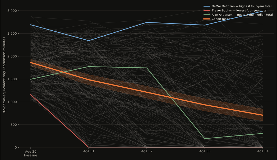
The players who disappear belong in the forecast
Let’s say we use only players who logged enough minutes at 34 years old to qualify for some performance metric we use for a model. We’re only looking at the “survivors” here, not the players who were injured, lost their spot in the rotation, or got caught cheating.
Depending on what analysis we’re performing and what the aim of that analysis is, we may want to use the conditional average. We might want to narrow our view to see how effective a player is given he’s able to remain in the rotation, for example.
For the Magic looking to hand Desmond Bane a hefty contract at age 31, it would be prudent to consider a world in which he is not a starting-caliber player for the duration of that contract.
The Magic should define the initial cohort for the analysis prior to the start of the forecast period. And, all of the players who qualify at the outset of the period should remain in the analysis, even those who lost roster spots or fell out of the league.
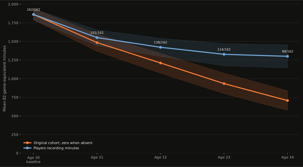
The two lines answer two different questions.
The survivor-only line asks how much work the remaining players handled. The full-cohort line asks how much work the original group provided. When evaluating an upcoming contract, you should not substitute the first line for the second.
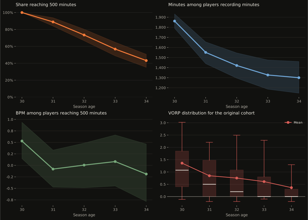
Availability vs effectiveness
The term “decline” can hold a variety of concepts with differing implications.
A player may keep his per-possession production in line with his historical averages, but play less minutes. Another player may remain available while moving into a smaller role. Yet another player might stay in his existing role, but produce less in this role over time.
The scenarios above, and countless more, all have different basketball explanations and mean something different for a roster.
The forecast should therefore separate at least three questions:
- What is the probability that the player remains available for an NBA role?
- How many minutes is he likely to play if available?
- How effective is he likely to be during those minutes?
A simple way to express the structure is:
E(total contribution) = P(available) × E(minutes × value per minute | available)
Obviously a simplification, but the above prevents a common interpretive error. A per-minute metric observed only for players who keep playing can’t represent the full downside of a multi-year deal.
Specificity is not better by default
Adding personal detail such as how they’ve responded to prior injuries or how their style of play has changed with age can make a projection sound more informed. Unfortunately, we can’t guarantee that the forecast will be improved with some extra detail alone.
When building out models, it’s always a good idea to start with start with a naive, or baseline, model. In our scenario, this would be a model that has no player-specific information beyond age and the cohort summary. Then test the player-specific model on seasons that were not used to fit it.
For starters, I would compare:
- An age-only cohort forecast.
- A forecast based primarily on the player’s recent trajectory.
- A partially pooled model combining the cohort with the player’s history + role.
- A more sophisticated model using additional basketball-related factors that were available at the time of the decision.
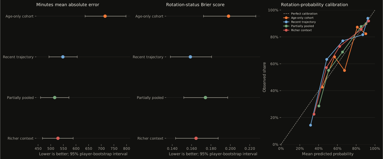
Different models may perform better for different scenarios. Maybe a naive model works better for players with less or more varied data. Maybe a more sophisticated model only outperforms for players beyond a certain age.
So what all should we consider when evaluating the contract?
Let’s now think about what the contract decision should include.
Per season of the upcoming contract, I would want to know:
- Expected total contribution
- Probability that the player remains in the intended role
- Probability of a major underachievement
- Reasonable upside & downside outcomes
- Which assumptions move those probabilities the most (a.k.a. feature importance)
- How much flexibility the contract leaves if the downside occurs (Taleb’s concept of “optionality”)
That last point is a key one. While not part of the aging curve model, it is hugely important for large contracts. Two player contracts that share identical expected basketball outcomes can expose a team to very different risks. Things like guarantees, options, incentives, and player and team options can all make or break a contract from a team’s perspective.
A wide range of outcomes is not a reason to avoid a contract. As is the case in finance, risk and reward go hand in hand. The potential upside of a player returning to form after a severe injury may be worth the risk to a team who finds their only plausible path to making the Finals via that potential outcome. In scenarios like this, contract terms and flexibility are very important.
The stat is not the decision
In the previous post about marginal and average possessions, the observed difference between paint-touch and no-paint-touch possessions did not tell us the value of creating one additional paint touch. We need to go several steps deeper to understand the counterfactuals and alternate paths.
The aging curve we’ve been discussing in this post presents a related problem. The average path provided by historical data doesn’t give us the full distribution of outcomes for a given player. Again, we need to go several steps deeper to understand who was included, who disappeared, the variance across individual careers, and how the player in question’s data reliably alters the predictions.
In the end, an aging curve certainly has its place in a contract evaluation. It would be a mistake to think you’ll be handing out that contract to the curve instead of the individual.
Analysis notes
The primary cohort contains 162 players who logged at least 1,000 82-game-equivalent regular-season minutes in an age-30 season from 2011–12 through 2021–22. Season age follows Basketball Reference. Every player remains in the panel through the next four seasons.
Minutes and games come from NBA.com. BPM, VORP, position, and season age come from Basketball Reference. A missing NBA season is zero minutes and zero VORP. It has no BPM value. “Active” means any recorded NBA minute; “rotation” means at least 500 adjusted minutes. The 2011–12, 2019–20, and 2020–21 schedules are scaled to an 82-game equivalent.
Intervals use 2,000 player-level bootstrap resamples. For model validation, each test prediction uses only outcomes completed by the end of that player’s baseline season. Hyperparameters and the partial-pooling weight are chosen within the earlier training data. Minutes models are compared by mean absolute error; rotation forecasts use the Brier score and grouped calibration. The test sample is small, so the observed ranking is not a guarantee that the same model will win for a future player.
| Age-30 minutes | Players | Any minutes at 34 | 500+ minutes at 34 | Mean minutes at 34 |
|---|---|---|---|---|
| 500 | 213 | 47% | 36% | 577 |
| 750 | 190 | 50% | 38% | 627 |
| 1,000 | 162 | 54% | 43% | 706 |
| 1,500 | 117 | 63% | 56% | 914 |
These are historical associations, not the causal effect of biological aging. Injury, role, team decisions, league selection, and era all contribute. The analysis is a cohort-level test, not a Desmond Bane contract forecast.
Sources: NBA.com traditional player statistics; Basketball Reference BPM and VORP methodology; NFL.com 2025 team passing statistics.